What is the pGM model?

The polarizable Gaussian Multipole (pGM) model combines distributed atomic charges, covalent dipoles, and induced dipoles. This note follows Wei et al. (2020), using the paper’s notation and equation numbers. We first consider a finite, nonperiodic system.

The logic is:

charge distribution → pair interaction → effective field → induced dipoles → energy and forces.

1. Gaussian monopoles and dipoles

Wei represents a monopole and a dipole centered at $\vec R$ as

\[ \begin{aligned} \rho^{(0)}(\vec r;\vec R) &=q\left(\frac{\beta}{\sqrt\pi}\right)^3 \exp\!\left(-\beta^2|\vec r-\vec R|^2\right),\\ \rho^{(1)}(\vec r;\vec R) &=\vec\mu\cdot\nabla_R \left(\frac{\beta}{\sqrt\pi}\right)^3 \exp\!\left(-\beta^2|\vec r-\vec R|^2\right). \end{aligned} \tag{2} \]

The Gaussian factor integrates to one, so the monopole has charge $q$. The dipole density has zero net charge and first moment $\vec\mu$. The Gaussian radius is $1/\beta$: decreasing $\beta$ spreads the distribution. The gradient $\nabla_R$ acts on the atomic center $\vec R$.

In the polarizable model, $q_i$ and $\vec\mu_i$ are the covalent charge and dipole on atom $i$, while $\vec p_i$ is its induced dipole. The combined dipole is written explicitly as $\vec\mu_i+\vec p_i$.

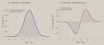
Figure 1. Analytical cross-sections of Eq. (2). The dipole is along the Cartesian x direction. Each density is divided by the scale shown on its vertical axis; the curves illustrate the functional form.

2. Pair interactions and effective fields

For atoms 1 and 2, Wei defines

\[ \beta_{12}=\frac{\beta_1\beta_2} {\sqrt{\beta_1^2+\beta_2^2}}, \qquad R^{12}=|\vec R_1-\vec R_2|. \tag{6} \]

The three pair interactions are

\[ q_1q_2\frac{\operatorname{erf}(\beta_{12}R^{12})}{R^{12}}, \tag{3} \] \[ q_1\vec\mu_2\cdot\nabla_2 \frac{\operatorname{erf}(\beta_{12}R^{12})}{R^{12}}, \tag{4} \] \[ (\vec\mu_1\cdot\nabla_1)(\vec\mu_2\cdot\nabla_2) \frac{\operatorname{erf}(\beta_{12}R^{12})}{R^{12}}. \tag{5} \]

These are the monopole–monopole, monopole–dipole, and dipole–dipole terms. Electrostatic conversion constants are suppressed. Following Wei’s operator convention, a gradient paired with a dipole differentiates the coordinate expression that follows, holding that dipole fixed during the operation.

The common factor approaches $1/R^{12}$ at large separation and $2\beta_{12}/\sqrt\pi$ at zero separation. The finite short-range value comes from integrating over the two distributed charge densities.

To express the interaction as a response to a field at atom 1, Wei introduces

\[ \begin{aligned} \phi^{effective} &=(q_2+\vec\mu_2\cdot\nabla_2) \frac{\operatorname{erf}(\beta_{12}R^{12})}{R^{12}},\\ \vec E^{effective} &=-(q_2+\vec\mu_2\cdot\nabla_2)\nabla_1 \frac{\operatorname{erf}(\beta_{12}R^{12})}{R^{12}}. \end{aligned} \tag{7} \]

Both atomic widths enter this effective potential and field. The real potential generated by atom 2 instead uses its source width alone:

\[ \phi^{real}=(q_2+\vec\mu_2\cdot\nabla_2) \frac{\operatorname{erf}(\beta_2R^{12})}{R^{12}}. \tag{8} \]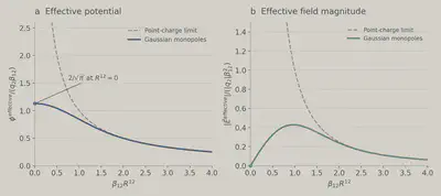

Figure 2. Eq. (7) for a monopole source, $\vec\mu_2=0$. The potential and field magnitude are scaled by $q_2\beta_{12}$ and $|q_2|\beta_{12}^2$, respectively. The abscissa is $\beta_{12}R^{12}$. The effective field magnitude vanishes at coincident centers and approaches the point-charge result at large separation.

3. Induced dipoles must be self-consistent

Wei’s polarization relation is

\[ \begin{aligned} \vec p_i&=\alpha_i\vec E_i^{effective}\\ &=\alpha_i\left(\vec E_i^{covalent,effective} -\sum_{j\ne i}\vec{\vec T}_{ij}\cdot\vec p_j\right),\\ \vec E_i^{covalent,effective} &=-\sum_{j\ne i}(q_j+\vec\mu_j\cdot\nabla_j)\nabla_i \frac{\operatorname{erf}(\beta_{ij}R^{ij})}{R^{ij}},\\ \vec{\vec T}_{ij}&=\nabla_i\nabla_j \frac{\operatorname{erf}(\beta_{ij}R^{ij})}{R^{ij}}. \end{aligned} \tag{10} \]

Here $\alpha_i$ is the atomic polarizability, and $\vec{\vec T}_{ij}$ is the dipole–dipole interaction tensor. Its mixed-derivative definition determines the minus sign in the induced field. Each $\vec p_i$ changes the fields driving the other dipoles, so evaluating only $\alpha_i\vec E_i^{covalent,effective}$ misses their mutual response. All induced dipoles must satisfy Eq. (10) together.

Following Wei, we now omit the superscript effective in the energy and force discussion. Thus $\vec E_i^{covalent}$ still denotes an effective field, and $\vec E_i$ includes both covalent and induced contributions. Gaussian screening removes the point-dipole singularity; stable polarization also depends on the chosen widths and polarizabilities (Elking et al.).

4. Covalent dipoles follow the molecular geometry

Wei also writes a covalent dipole as $\vec u$ when expressing it in a covalent basis vector (CBV) frame. This is the same permanent dipole represented by $\vec\mu$ above. For one atom,

\[ \nabla(\vec u) =\nabla\left(\sum_i u_i\frac{\vec R_i}{|\vec R_i|}\right) =\sum_i u_i\left( \frac{\vec{\vec I}}{|\vec R_i|} -\frac{\vec R_i\vec R_i}{|\vec R_i|^3}\right). \tag{9} \]

In this local expression, $\vec R_i$ points from the atom whose dipole is being defined to its ith covalently interacting neighbor, including virtual neighbors. The $u_i$ are fixed coefficients, and $\vec{\vec I}$ is the identity tensor. This local use of $\vec R_i$ follows Wei’s Eq. (9); elsewhere, $\vec R_i$ denotes an atomic position.

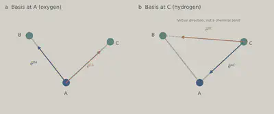
Figure 3. A is oxygen; B and C are hydrogens, as in Wei’s Fig. 1. At A, the basis vectors are $\vec e^{BA}$ and $\vec e^{CA}$. At C, they are $\vec e^{AC}$ and $\vec e^{BC}$. The second superscript identifies the origin: $\vec e^{BA}$ points from A toward B. The dashed C–B segment defines a virtual direction. Geometry is schematic.

The CBVs move as the molecule moves. Their geometry dependence in Eq. (9) must therefore enter the force calculation.

5. Energy, the factor one-half, and forces

Wei separates the electrostatic energy into the covalent interaction energy and the induced energy. For $N$ atoms, the first part is

\[ \begin{aligned} U_{covalent-covalent} ={}&\frac12\sum_i^N\sum_{j\ne i}^N (q_i+\vec\mu_i\cdot\nabla_i) (q_j+\vec\mu_j\cdot\nabla_j)\\ &\hspace{3em}\times \frac{\operatorname{erf}(\beta_{ij}R^{ij})}{R^{ij}}. \end{aligned} \tag{13} \]

Linear polarization requires the single-atom self-energy

\[ U=\frac12\frac{\vec p^{2}}{\alpha}. \tag{11} \]

The induced energy contains induced–covalent interactions, induced–induced interactions, and this self-energy. At self-consistency, $\vec p_i/\alpha_i=\vec E_i^{covalent} -\sum_{j\ne i}\vec{\vec T}_{ij}\cdot\vec p_j$. Substituting this relation into the self-energy gives Wei’s cancellation:

\[ \begin{aligned} U_{induced} ={}&U_{induced-covalent}+U_{induced-induced}+U_{self}\\ ={}&-\sum_i^N\vec p_i\cdot\vec E_i^{covalent} +\frac12\sum_i^N\sum_{j\ne i}^N \vec p_i\cdot\vec{\vec T}_{ij}\cdot\vec p_j\\ &+\frac12\sum_i^N\vec p_i\cdot\left( \vec E_i^{covalent} -\sum_{j\ne i}^N\vec{\vec T}_{ij}\cdot\vec p_j\right)\\ ={}&-\frac12\sum_i^N\vec p_i\cdot\vec E_i^{covalent}. \end{aligned} \tag{14} \]

The two induced–induced sums cancel, leaving the factor $1/2$. The final line applies to self-consistent dipoles. During an unconverged iteration, the self-energy remains $\tfrac12\sum_i\vec p_i^{2}/\alpha_i$; the shortened final line is not the energy functional away from the solution. Wei distinguishes this polarization self-energy from the Coulomb assembly energy of a Gaussian density in Eqs. (11)–(12).

After accounting for moving covalent dipoles and the induced response, Wei expresses the total force in terms of fields and field gradients:

\[ \vec F^{i} =\sum_j^n\nabla_i(\vec u_j)\cdot\vec E_j +q_i\vec E_i +(\vec u_i+\vec p_i)\cdot\vec{\vec E}_i. \tag{39} \]

Here $n$ covers the atoms that covalently interact with atom $i$, including its own dipole when geometry-dependent. The tensor $\vec{\vec E}_i$ is the field gradient, with covalent and induced contributions as defined in Wei’s Eq. (32). The first term carries the CBV geometry derivatives; the remaining terms couple the charge and total dipole to the field and its gradient.

6. From equations to molecular dynamics

At each geometry: build the CBV frames, evaluate covalent fields, solve Eq. (10) self-consistently, then evaluate energy and forces. For periodic systems, PME supplies the long-range sums. Wei denotes the Ewald splitting parameter by $\beta_0$; it is a numerical parameter distinct from the atomic widths $\beta_i$.

Wei checked analytical forces against finite differences for a water dimer and tested energy conservation in a 512-water NVE simulation. Both induction convergence and PME accuracy matter for these calculations. Parameter development is a separate task; see Wang et al. (2019) for atomic polarizability and anisotropy.

References and scope

The mathematical derivations and figures here are explanatory. Figures 1–2 evaluate analytical expressions; Figure 3 is a schematic. None reproduces simulation data from the cited papers.

1. Wei, H.; Qi, R.; Wang, J.; Cieplak, P.; Duan, Y.; Luo, R. Efficient formulation of polarizable Gaussian multipole electrostatics for biomolecular simulations. J. Chem. Phys. (2020). Publisher article · Author preprint. Equation references above follow the author preprint.
2. Elking, D.; Darden, T.; Woods, R. J. Gaussian induced dipole polarization model. J. Comput. Chem. 28, 1261–1274 (2007). Publisher article.
3. Wang, J.; Cieplak, P.; Luo, R.; Duan, Y. Development of Polarizable Gaussian Model for Molecular Mechanical Calculations I: Atomic Polarizability Parameterization To Reproduce ab Initio Anisotropy. J. Chem. Theory Comput. 15, 1146–1158 (2019). Publisher article.